Creation and manipulation of quantized vortices in Bose-Einstein condensates using reinforcement learning

I came cross the work Creation and manipulation of quantized vortices in Bose-Einstein condensates using reinforcement learning a few months ago and found it quite interesting.

In this work, the author uses reinforcement learning to control the quantum dynamics of a non-linear Bose-Einstein condensates (BECs). A reinforcement-learning-based optimization of quantum control of a superconducting qubit system is discussed in a previous note AlphaZero explores global optimization of quantum dynamics in superconducting circuit QED. Personally, I believe that cold atom systems like BECs provide accessible platforms for testing machine learning algorithms in physics since the order parameter of the condensate is nothing but a linear superposition of different plane-wave states. Especially, higher-momentum or higher-energy states are less likely to be involved in most physical processes. The BEC basically states a fairly less complicated nonlinear system even with contact interaction or dipolar interaction.

Model and Method

The author considers a simple model, where a trapped BEC with contact interaction is subject to a Gaussian potential so that its effective Hamiltonian reads
$$\mathcal{H}=-\frac{\hbar^2}{2m}\nabla^2+V_{trap}+V_G+g\vert\psi\vert^2$$
, where $V_{trap}$ represents a harmonic trap and $V_G$ is the time-dependent Gaussian potential. Here, the author assumes that both the amplitude $A(t)>0$ and centers $\xi(t)$ and $\eta(t)$ along $x$ and $y$ are control parameters.

The reinforcement learning process can be summarized as following. The environment is basically the BEC simulator (numerical simulation of GP equation), which takes input as the the Gaussian potential profile in time domain and outputs the final state of the BEC. The agent is then fed with BEC order parameters (specifically, the density distribution $\vert\psi\vert^2$ and flux distribution $\psi^\ast\nabla\psi-\psi\nabla\psi^\ast$) as well as corresponding rewards and take actions to obtain a new control signal. The agent is trained to optimize the reward function (namely, the absolute value of overlap integral between current state and target state), leading to the desired preparation of any state of the BEC.

Learning algorithm

For the agent, it gets the reward $r_t$ from the environment (the simulator), which is computed using the current state $s_t$, and determines the action $a_t$ on the environment. The agent aims to minimize the discounted cumulative reward $\sum_n\gamma^nr_{t+n\Delta t}$, where $0<\gamma<1$ is the discount rate and $\Delta t$ is time-evolution step.

The real space is sampled by 64 $\times$ 64 points and the density distribution, the flux and the Gaussian potential are fed into a deep convolutional neural network (CNN) with four convolutional layers and two fully-connected layers. The CNN outputs six values $Q(s_t,a),a=0,1,…,5$ and the agent determines the action $a_t$ through a $\epsilon$-greedy policy. Namely, it generates a radom number $0\leq r<1$ and take a random choice if $r<\epsilon$, otherwise, the agent takes the action $a$ with maximum $Q(s_t,a)$. It is clear that $\epsilon$ determines the level of explorations. In the implementation, $\epsilon$ is linearly decreased from 1 to 0.1 in the first 50000 steps and remains a constant afterwards. In practice, the six possible actions are $\xi\to\xi\pm\delta\xi$, $\eta\to\eta\pm\delta\eta$ and $A\to A\pm\delta A$.

The training process of the CNN is followed. A queue of 50000 sets of data $(s_t,a_t,r_t,s_{t+\Delta t})$ is maintained. Once the queue reaches its maximum length, 32 sets of data are taken randomly and the network is trained using gradients of Huber loss. The author keeps two copies of the CNN, the origin one is used to generate $Q$ and it is copied to a target CNN every 1000 steps. The target CNN is used to update the Huber loss in the training process.

The author also kindly includes a pseudocode in the work to describe the algorithm, which is fairly easy to follow.

Results

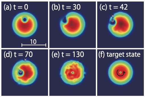
Finally, the author applies the algorithm and good results for both 2D and 3D systems. The author focuses on the preparation of vertex state but it looks like the method is general for other states. However, it looks like in 2D, the final states obtained by the agent is not in perfect agreement with the target state. I suspect that on one hand, the learning algorithm remains to be optimized and on the other hand, this is a dynamical process after all and the author only allows 500 steps towards to the final state. It’s also unclear how non-linear interactions affects the performance of the algorithm.

Reference

• Creation and manipulation of quantized vortices in Bose-Einstein condensates using reinforcement learning
• GP equation - Wikipedia