AlphaZero explores global optimization of quantum dynamics in superconducting circuit QED

I’ve been thinking about a class of optimization problems on a quantum computer and wish to explore them with machine learning algorithms, especially reinforcement learning, as it does not require a good initial guess (radom, intuition or whatever). More recently, I came across to the paper “Global optimization of quantum dynamics with AlphaZero deep exploration”, which has been published online about 2 weeks ago. While the authors considered a rather ideal situation, their work did shed lights on my research. So, I prepare this note to briefly discuss their work and some relevant topics.

Background

Quantum control is basically to design a series of control signals, which transfer a quantum system from an initial state $\left|i\right\rangle$ to a given final state $\left|f\right\rangle$. If you ever learned a little bit quantum mechanics, you would probably know the adiabatic theorem and may think less of quantum control theory. However, adiabatic process is not realistic in experiments and real-life applications due to underlying constraints (e.g. unreachable parameter space, limited control time). Not to mention that there’s no adiabatic limit in Anderson/many-body localized or Floquet (periodically driven) systems. Quantum optimal control theory has raised for designing control signals of stimulated system.

Under ideal physical conditions, it has been shown that local exploitation is sufficient for ultimate optimization. This is a result of “perfect” landscape of the transition probability $P_{i\to f}=\vert\langle i\vert U(C(t))\vert f\rangle\vert^2$, where $U(C(t))$ is the unitary transformation determined by the control signal $C(t)$. Previous works have proven that when the quantum state of interest is finite, the functional $\delta P_{i\to f}/\delta C(t)=0$ has at least one solution so that $P_{i\to g}=1$. Then, there is no suboptimal local extrema as long as there’s no extra constraint.

As discussed before, this is not realistic and in fact, imposing significant constraints on the dynamics may make the optimization problem as hard as “NP-complete” problems (I’m not 100% certain about this). Besides the optimal control methods, reinforcement learning with deep neural network (DNN) has been applied to optimize dynamically evolving systems. More recently, the AlphaZero algorithms have shown great breakthrough in playing games like Go and Starcraft. AlphaZero combines Monte Carlo tree search (MCTS) with a one-step lookahead DNN, leading to more focused and heuristic-independent explorations.

AlphaZero explores optimization of quantum dynamics

Physical model

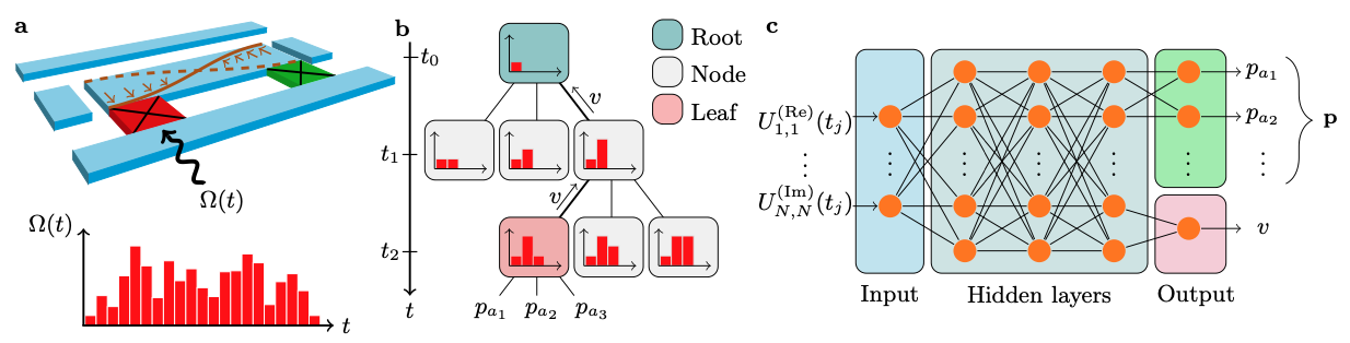
The authors consider a two-transmon system with cross-resonance gate, whose dynamics is govern by the Hamiltonian $H=\Delta b_1^\dagger b_1+J(b_1^\dagger b_2+ h.c.) + \Omega(t)(b_1^\dagger+b_1)$, where $\Delta/2\pi=0.35$ GHz is detuning, $J/2\pi=5$ MHz is qubit coupling constant and $\Omega(t)$ denotes the control field. The $b_i,i=1,2$ is the qubit-lowering operator. I also write here, the corresponding matrix form in computational basis for convenience
$$H = \begin{pmatrix} 0 & 0 & 0 & \Omega(t) \\ 0 & 0 & J & 0 \\ 0 & J & \Delta & 0 \\ \Omega(t) & 0 & 0 & \Delta \end{pmatrix}.$$

The criteria/rewards function here is clearly the fidelity, defined as $\vert\frac{1}{\text{dim}}\text{Tr}\left[U^\dagger(t)U_f\right]\vert^2$, where $U_f$ is the target unitary. In this work, the authors consider an entangling gate
$$U_f=\sqrt{\sigma_z\sigma_x}=e^{(-i\frac{\pi}{4}\sigma_x\sigma_z)} = \begin{pmatrix} 1 & -i & 0 & 0 \\ -i & 1 & 0 & 0 \\ 0 & 0 & 1 & i \\ 0 & 0 & i & 1 \end{pmatrix}.$$
Note that, once a particular $\Omega(t)$ is given, the corresponding unitary can be solved by simulating quantum time evolution.

The AlphaZero implementation

We refer to a successful generation of a pulse sequence as an episode and the agent wants to maximize the fidelity at the end of each episode. Again, the AlphaZero algorithm can be considered as a MCTS, guided by a one-step lookahead NN. We discuss each part in the following.

Monte Carlo tree search

If you are not familiar with MCTS, please refer to Wiki - MCTS for a basic introduction.

Once we discretize the time, we may treat the signal as a time series. Such a sequence represents a state $s_i$ at time $t_i,i=0,1,2,…,N$. To implement the MCTS, we take a possible state as node and parent/child nodes are connected by edges, which contain important information including a visit count $N(s_i,a_i)$, a total action value $W(s_i,a_i)$, a mean action value $Q(s_i,a_i)$ and a prior probability $P(s_i,a_i)$.

Initially, the tree has only a root with the state being identity matrix at $t_0$ (nothing has been done on the system at $t_0$). The probabilities $P(s_t,a_t)$ are initialized with the NN outputs while others are set as zero $N(s_t,a_t)=W(s_t,a_t)=Q(s_t,a_t)=0$.

At the expansion stage, the authors introduce an uncertainty $U(s_c,a_j)=c_pP(s_c,a_j)\frac{\sqrt{\sum_iN(s_0,a_i)}}{1+N(s_c,a_j)}$ to help them select the action under current state $s_c$. Specifically, the next action is given by max$({Q(s_c,a_j)+U(s_c,a_j)})$. Note that, $c_p$ determines the level of exploration in the sense that the algorithm tends to take less visited action with larger $c_p$. $c_p=1$ is set in this work. Now, the expansion is repeated until we encounter a new leaf node.

Once we arrive at a new leaf $s_n$, we feed the current unitary into NN to get outputs $(p, v)$. We initialize all the edges of this leaf as before, namely, $P(s_n,a_t)=p$ ($p$ is generally a vector) and $N(s_n,a_t)=W(s_n,a_t)=Q(s_n,a_t)=0$. After this is done, we have to do back-prorogations for all the parent state $s_r$ involved, following $N(s_r,a_r)++$, $W(s_r,a_r)+=v$ and $Q(s_r,a_r)=W(s_r,a)/N(s_r,a_r)$.

Once a pre-set number of searches is reached, we generate a policy for current root $s_t$ using the visit count $\pi(a_j\vert s_t)=\frac{N(s_t,a_j)^{(1/\tau)}}{\sum_iN(s_t,a_i)^{1/\tau}}$, where $\tau$ is also a hyperparameter that governs the level of exploration. In their work, the authors hyperbolically anneal it from 1 to 0.001 with a rate of 0.001. The authors also take a deterministic policy by choosing the maximum when $\tau<0.9$. Once an action is drawn by the policy, the root $s_t$ is cached and one of its child state (namely, the chosen one) becomes the new root and all other children are discarded or dumped.

The above procedure is repeated until we have a new full control sequence in the cache and then, one episode is done. In their implementations, the authors cut the branches, which have been fully explored in previous episodes, to improve efficiency.

Neural network

The NN takes the unitary $U(t)$ as input and outputs the possibilities $p$ for each possible movement and an estimate of final fidelity $v$. The NN is initialized randomly and is only trained after one episode is completed.

In this work, the authors choose a simple feed forward network, in which there are 4 hidden layers, each containing 400 nodes, followed by batch normalization and a rectified linear unit. The L2 regularization parameter is 0.001 and they apply Dirichlet noise to the probability $P(s,a)=(1-\epsilon)p_a + \epsilon \eta_a$, where $\eta\sim\text{Dir}(0.03)$ and $\epsilon=0.25$.

Results

The results can be easily understood through Figs. 2-4 in the paper and AlphaZero indeed showcases great performances. Here, I only remarked some important aspects of two studied cases.

Digital gate sequences

In this case, the control signal is simply Gaussian pulse $\Omega(t)=\frac{a}{\sqrt{2\pi}\tau}e^{-\frac{(t-\Delta t/2)^2}{2\tau^2}}$, where $\tau=0.25$ ps, $\Delta t=2.0$ ps and $a=2\pi/1000$. The pulse series can be represented by a string of 0 and 1.

The gate duration is typically around 50 ns, which contains $10^4$ to $10^5$ signals.

Constrained analogy pulses

Analogy pulse is a little bit tricky. The authors sample the amplitude of the beam by 60 points and consider the bandwidth constraint via a convolution with a Gaussian filter function $\Omega’(t)=\int e^{\frac{(t-t’)^2}{\sigma^2}}\Omega(t’)dt’$. The maximum amplitude is chosen as $\Omega/2\pi=1.0$ GHz and $\sigma=0.7$ ns.

Reference

• Global optimization of quantum dynamics with AlphaZero deep exploration
• Quantum optimally controlled transition landscapes
• Reinforcement Learning in Different Phases of Quantum Control

Reference - AlphaZero

• Mastering the game of Go with deep neural networks and tree search
• Mastering the game of Go without human knowledge
• A general reinforcement learning algorithm that masters chess, shogi, and Go through self-play